Basic Application Architecture
Developer Perspective
A typical application is composed of:
- Build & Deploy Layer, CI/CD pipeline
- Server Layer, handles incoming requests
- Storage Layer, persists application data (can be external)
- Logging Storage Server, logs all events
- Metric Storage Server, logs all metrics
- Alert Server, alerts when something goes down
Stateless vs Stateful Services
- Stateless: the server holds no session data between requests. Any instance can serve any request. Enables effortless horizontal scaling.
- Stateful: the server holds session data (e.g. WebSocket connections, in-memory cart). Requires sticky sessions (session affinity at the load balancer) or externalizing state to Redis/a DB.
| Stateless | Stateful | |
|---|---|---|
| Horizontal scaling | Trivial, add instances freely | Hard, requires sticky sessions or external state |
| Fault tolerance | High, any replica serves the request | Low, losing a server loses its session data |
| Examples | REST APIs, static servers | WebSocket servers, game servers, video call nodes |
User Perspective
Users simply make requests to the server and receive responses.
System Architecture Overview
graph LR
    User -->|HTTPS| CDN
    CDN -->|Cache Miss| LB[Load Balancer]
    LB --> App1[App Server 1]
    LB --> App2[App Server 2]
    LB --> App3[App Server 3]
    App1 --> Cache[(Redis Cache)]
    App2 --> Cache
    App3 --> Cache
    Cache -->|Cache Miss| DB[(Primary DB)]
    DB --> Replica1[(Read Replica 1)]
    DB --> Replica2[(Read Replica 2)]
Single Points of Failure
| Layer | SPOF risk | Mitigation |
|---|---|---|
| Server | Single app server fails → full outage | Horizontal scaling + load balancer |
| Load balancer | LB fails → full outage | Active-active LB pair with floating IP (VRRP) |
| Database | Single DB fails → data unavailable | Primary + read replicas, automatic failover |
| Storage | Single disk fails → data loss | RAID, object storage with replication (S3 11-nines durability) |
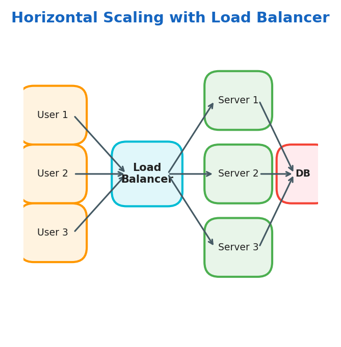
Scaling
- Vertical Scaling: add more physical resources (CPU, RAM) to a single server
- Horizontal Scaling: add more servers to distribute the load
- Load Balancer: distributes traffic between multiple servers
Vertical Scaling Limits
⚠️ Warning: Vertical scaling has a hard ceiling. The largest cloud instances (e.g. AWS
u-24tb1.metal) top out at ~448 vCPUs and 24 TB RAM and cost thousands of dollars per hour. Beyond that, horizontal scaling is the only option.
Design Requirements
How We Handle Data
| Concern | Description |
|---|---|
| Move data | Data moves between servers in different parts of the world |
| Store data | How we persist our data |
| Transform data | Transforming data to answer queries or perform computations |
Metrics for Evaluating Our Design
Availability, measures uptime of a system:
$$\text{Availability} = \frac{\text{uptime}}{\text{uptime} + \text{downtime}}$$Example:
$$\frac{23 \text{ hours}}{23 \text{ hours} + 1 \text{ hour}} = 96\%$$| Availability | Downtime per year | Downtime per month |
|---|---|---|
| 99% (“two nines”) | ~3.65 days | ~7.3 hours |
| 99.9% (“three nines”) | ~8.77 hours | ~43.8 minutes |
| 99.99% (“four nines”) | ~52.6 minutes | ~4.4 minutes |
| 99.999% (“five nines”) | ~5.26 minutes | ~26 seconds |
💡 Tip: Each additional nine is roughly 10× harder to achieve. Going from 99.9% to 99.99% often requires redundant infrastructure, active-active deployments, and chaos engineering.
SLI / SLO / SLA, worked example:
SLI  = (successful requests / total requests) × 100
SLO  = "API availability SLI ≥ 99.9% over a rolling 30-day window"
SLA  = contract: if SLO is breached, customer receives 10% service credit
Error Budget
The error budget is the allowed failure quota derived directly from the SLO:
$$\text{Error Budget} = 1 - \text{SLO} = 1 - 0.999 = 0.001 = 43.8 \text{ min/month}$$Assuming a 30.44-day average month (\(365.25/12\)): \(0.001 \times 30.44 \times 24 \times 60 \approx 43.8\) minutes (rounded to one decimal place).
- Teams spend the error budget on deployments, experiments, and planned maintenance.
- When the budget is exhausted, all risky changes freeze until the window resets.
- This creates a healthy tension between reliability (SRE) and feature velocity (Dev).
Reliability, measures the probability of a system failing
Reliability
$$\text{MTBF} = \frac{\text{Total uptime}}{\text{Number of failures}} \qquad \text{MTTR} = \frac{\text{Total downtime}}{\text{Number of failures}}$$$$\text{Availability} = \frac{\text{MTBF}}{\text{MTBF} + \text{MTTR}}$$Improving availability means either increasing MTBF (fewer failures, better code, hardware) or decreasing MTTR (faster recovery, better alerting, runbooks, auto-remediation).
Fault Tolerance, measures how much our system can continue working under failure
Redundancy, measures how much our system is replicated
Throughput, measures the number of operations in a time frame:
$$\text{Throughput} = \frac{\text{operations}}{\text{time}} = \frac{\text{queries}}{\text{seconds}} = \frac{\text{bytes}}{\text{seconds}}$$Latency, measured as a percentile distribution, not a mean:
| Percentile | Meaning |
|---|---|
| p50 (median) | Half of requests are faster than this |
| p95 | 95% of requests are faster than this |
| p99 | 99% of requests are faster than this, what most users experience at the tail |
| p999 | 1-in-1000 requests, the “long tail” that affects your biggest/most active users |
💡 Tip: Always design to a p99 target, not a mean. A mean of 50ms can hide a p99 of 2,000ms. Users at the tail are often your highest-value customers (power users making the most requests).
Networks
Basics
| Concept | Description |
|---|---|
| Packages | Encapsulate data to be transferred over the network |
| IP Address | Virtual identification of a host |
| MAC Address | Physical identification of a host |
| NAT | Translates public IP to private within a LAN. Devices in a LAN have their own private IPs and access the internet using a single public IP |
| Port Forwarding | Network technique that enables external users to access specific services on a private, local network |
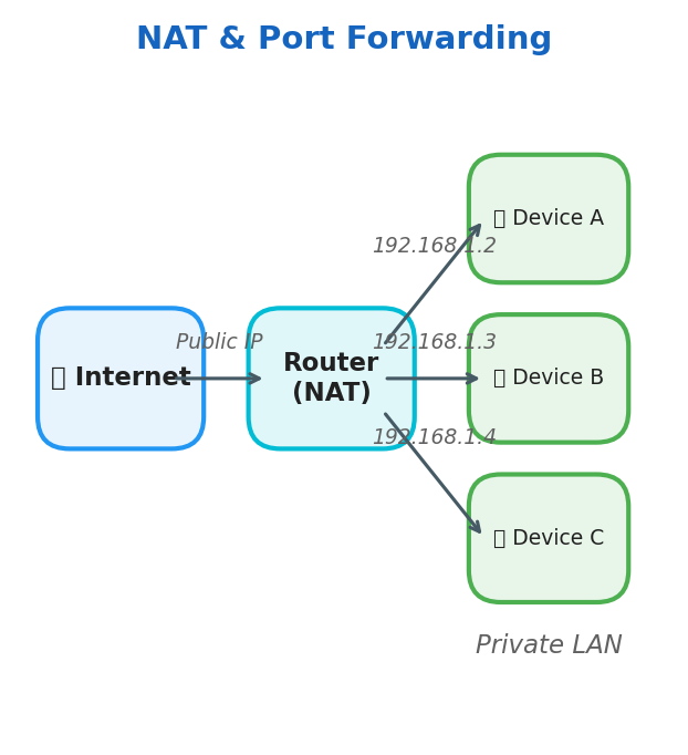
Router, sends packages across the network
Basic Protocols
| Protocol | Description |
|---|---|
| HTTP | Exchange hyper-text information |
| SSH | Remote connection to a host |
| TCP | Stateful communication, 3-way handshake, congestion handling, retransmission of lost packages |
| UDP | Non-stateful communication, no guarantees |
💡 Tip: Use UDP for real-time applications (video calls, games) where occasional packet loss is acceptable but latency must be minimal. Use TCP when every byte must arrive in order (file transfers, APIs).
TCP Three-Way Handshake
Every TCP connection requires 1 full round-trip before data can flow:
sequenceDiagram
    participant C as Client
    participant S as Server
    C->>S: SYN (seq=x)
    S->>C: SYN-ACK (seq=y, ack=x+1)
    C->>S: ACK (ack=y+1)
    Note over C,S: Connection established, data transfer begins
Cost implications:
- 1 RTT overhead per new TCP connection
- HTTPS adds another 1-2 RTTs for the TLS handshake on top
- This is why connection pooling and HTTP/2 multiplexing matter so much at scale
💡 Tip: Connection pooling (PgBouncer for Postgres, HikariCP for Java) amortises the TCP + TLS handshake cost across many requests. At scale, a fresh TLS handshake per request can cost 50–100ms, more than the query itself.
DNS Resolution
DNS translates human-readable hostnames into IP addresses. The resolution chain:
sequenceDiagram
    participant B as Browser
    participant R as Recursive Resolver (ISP)
    participant Root as Root Nameserver
    participant TLD as TLD Nameserver (.com)
    participant Auth as Authoritative NS (example.com)
    B->>R: resolve api.example.com
    R->>Root: who handles .com?
    Root->>R: TLD NS address
    R->>TLD: who handles example.com?
    TLD->>R: Authoritative NS address
    R->>Auth: what is api.example.com?
    Auth->>R: 93.184.216.34 (TTL: 300s)
    R->>B: 93.184.216.34 (cached for 300s)
Key system design implications:
- TTL controls propagation delay, low TTL = faster failover, higher DNS load; high TTL = slower failover, less load
- GeoDNS, return different IPs based on the requester’s geographic location (closest region)
- DNS-based load balancing, return multiple A records; clients round-robin. Simple but no health checks.
TLS Handshake
TLS adds encryption, authentication, and integrity on top of TCP. Modern TLS 1.3 takes 1 RTT (vs 2 RTTs for TLS 1.2):
- ClientHello, client sends supported cipher suites, TLS version, random nonce
- ServerHello + Certificate, server chooses cipher, sends its X.509 certificate
- Key Exchange, both sides derive the same session key using ECDHE (no key transmitted)
- Finished, both sides confirm encryption is working; data flow begins
💡 Tip: TLS termination at a load balancer means internal traffic is unencrypted. For regulated industries (healthcare, finance), use mTLS (mutual TLS) internally so every service authenticates both directions.
HTTP/1.1 vs HTTP/2 vs HTTP/3
| Feature | HTTP/1.1 | HTTP/2 | HTTP/3 |
|---|---|---|---|
| Transport | TCP | TCP | QUIC (UDP) |
| Multiplexing | No, one request per connection | Yes, multiple streams per connection | Yes |
| Head-of-line blocking | Per-connection | TCP-level (one lost packet stalls all streams) | Eliminated, per-stream |
| Header compression | None | HPACK | QPACK |
| Connection setup | TCP + TLS = 2 RTT | TCP + TLS = 2 RTT | 0-RTT possible |
| Best for | Legacy systems | Most modern APIs | Mobile, lossy networks |
📖 Deep Dive: HTTP/3 and QUIC are defined in RFC 9000. Cloudflare’s blog has an excellent series on their real-world QUIC deployment.
API Design
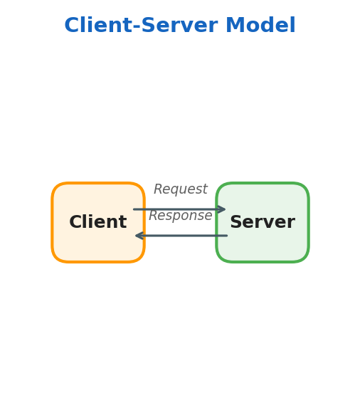
Client-Server Model
- Client, accesses information provided by a server
- Server, provides resources
RPC, Remote Procedure Call
The RPC model allows a program to execute code in a different machine or address space.
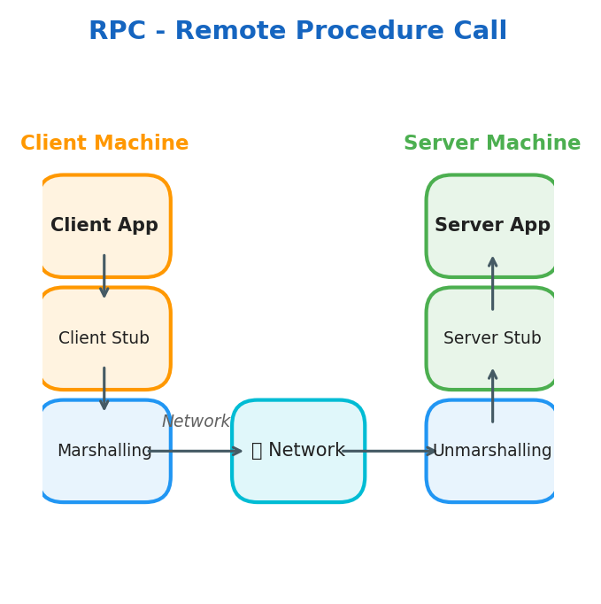
Key concepts:
- Stub, function proxy on both local and remote server
- Marshalling, packaging parameters into a message ready to be sent
- Unmarshalling, unpacking parameters from the received message
HTTP / HTTPS
HTTP is the protocol for client-server communication. TLS/SSL encrypts traffic between client and server.
Methods:
| Method | Purpose |
|---|---|
| GET | Retrieve resources |
| POST | Create resources |
| PUT | Update/replace resources |
| DELETE | Remove resources |
Status Codes:
| Range | Meaning |
|---|---|
| 1xx | Informational |
| 2xx | Successful |
| 3xx | Redirection |
| 4xx | Client Error |
| 5xx | Server Error |
Cons: HTTP is not ideal for real-time data exchange
WebSockets
WebSockets establish a persistent, full-duplex connection between client and server, unlike REST where each request creates a new connection.
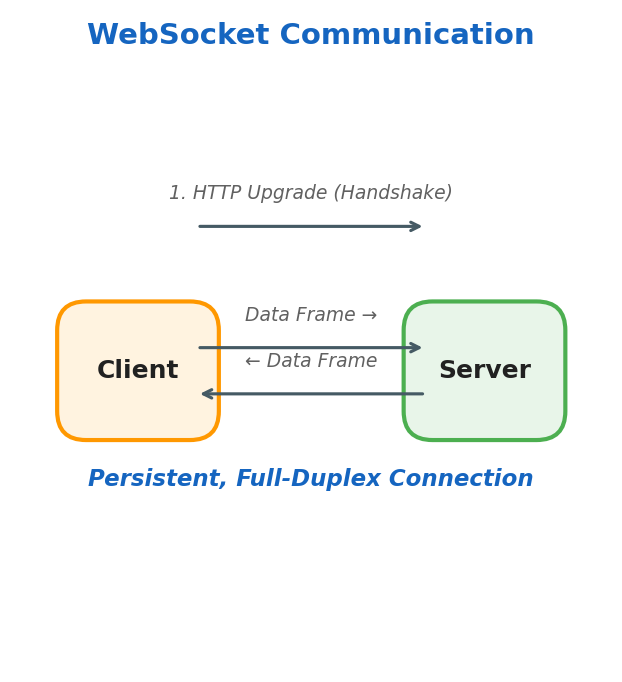
Pros:
- Bi-directional communication
- Great for real-time data (chat, live feeds)
- Supports server push and polling
API Paradigms
REST
- Stateless, server doesn’t maintain session state
- Pagination, page through resources
- Cacheable, responses can be cached
- Resource-identified, resources have unique URIs, exchanged in JSON
- Layered, client and server are decoupled; can talk to replicas transparently
GraphQL
GraphQL lets clients request exactly the data they need, no over-fetching (getting unused fields) or under-fetching (needing multiple requests for related data).
The N+1 Query Problem, GraphQL’s most common performance trap:
# Naive resolver, fires 1 DB query per user (N+1 total)
def resolve_posts(root, info):
    posts = db.query("SELECT * FROM posts")          # 1 query
    for post in posts:
        post.author = db.query(                       # N queries
            "SELECT * FROM users WHERE id = ?",
            post.author_id
        )
    return posts
Solution: DataLoader, batches all author lookups into a single SELECT * FROM users WHERE id IN (...) query.
| REST | GraphQL | gRPC | |
|---|---|---|---|
| Protocol | HTTP/1.1+ | HTTP/1.1+ | HTTP/2 |
| Data format | JSON | JSON | Protobuf (binary) |
| Schema | OpenAPI (optional) | SDL (required) | .proto (required) |
| Type safety | Weak | Strong | Strong |
| Caching | HTTP cache (GET) | Hard (POST only) | Custom |
| Browser support | Native | Native | Needs gRPC-Web |
| Best for | Public APIs | Complex client needs | Internal microservices |
| Streaming | SSE / WebSocket | Subscriptions | Native bi-directional |
gRPC
- Typically used for server-to-server communication
- Implements RPC with schema-defined data
- Faster than REST
- Supports bi-directional streaming
- Uses exceptions instead of status codes
- Built on HTTP/2
Cons:
- No native browser support, requires gRPC-Web proxy (Envoy) or gRPC-Web library
- Binary protocol, harder to debug than JSON (need protoc or grpcurl)
- Schema evolution rules, never change field numbers; only add new fields; deprecate with
reserved - Tight coupling, both sides must share the
.protoschema file
API Design Best Practices
API Contract, defines the structure of your API
Handling API changes:
- Adding parameters → make them optional
- Removing parameters → can break external customers
Pagination, limit the number of returned objects:
GET https://api.example.com/v1/users/:id/tweets?limit=10&offset=0
HTTP Idempotency, making the same request multiple times produces the same effect:
| Method | Idempotent? |
|---|---|
| GET | ✅ Yes |
| PUT | ✅ Yes |
| DELETE | ✅ Yes |
| POST | ⚠️ Depends on implementation |
Rate Limiting
Rate limiting protects backend services from abuse and accidental overload.
Common algorithms:
- Token Bucket, tokens refill at a fixed rate; requests consume tokens. Allows short bursts.
- Leaky Bucket, requests are processed at a fixed rate; excess requests are queued or dropped. Smooths output traffic.
- Fixed Window, count requests per time window (for example, 1000 req/min). Simple but vulnerable to boundary bursts.
- Sliding Window, tracks requests over a rolling window. More accurate than fixed windows, but uses more memory.
Practical selection guidance:
- Token Bucket when APIs must tolerate short bursts without overwhelming downstream systems.
- Leaky Bucket when you need steady outbound flow to protect a constrained backend.
- Fixed Window when implementation simplicity matters more than strict fairness.
- Sliding Window when enforcement accuracy is more important than memory overhead.
When clients exceed limits, return 429 Too Many Requests with a Retry-After header.
Common implementations include NGINX rate limiting, Redis + Lua scripts, and API Gateway products such as Kong and AWS API Gateway.
Authentication & Authorisation
| Pattern | How it works | Best for |
|---|---|---|
| API Key | Static secret in header (X-API-Key) | Server-to-server, simple integrations |
| Basic Auth | Base64(user:pass) in Authorization header | Legacy, internal tools (always over HTTPS) |
| OAuth2 + OIDC | Token-based delegated access, refresh tokens | Third-party login, user-facing apps |
| JWT | Self-contained signed token; no DB lookup to verify | Stateless APIs, microservices |
| mTLS | Both client and server present certificates | Internal service-to-service (zero trust) |
JWT structure:
header.payload.signature
// Header
{ "alg": "RS256", "typ": "JWT" }

// Payload (claims, do NOT store sensitive data, it's only base64-encoded)
{ "sub": "user-123", "roles": ["admin"], "exp": 1742000000 }

// Signature = RS256(base64(header) + "." + base64(payload), private_key)
sequenceDiagram
    participant C as Client
    participant A as Auth Service
    participant R as Resource API
    C->A: POST /login (credentials)
    A->C: access_token (15min) + refresh_token (7d)
    C->R: GET /api/data (Bearer access_token)
    R->R: Verify JWT signature (no DB call)
    R->C: 200 OK + data
    Note over C,R: 15 minutes later...
    C->A: POST /refresh (refresh_token)
    A->C: new access_token
⚠️ Warning: JWTs cannot be revoked before expiry without a token blocklist (Redis set of revoked JWT IDs; token identifier claim =
jti). Keep access token lifetime short (15 min) and use refresh tokens for renewal.
📖 Deep Dive: Read RFC 7519 for the JWT spec and oauth.net for the full OAuth2 framework.
API Versioning
| Strategy | Example | Pros | Cons |
|---|---|---|---|
| URL versioning | /v1/users | Explicit, easy to route | Proliferates versions in URL |
| Header versioning | Accept: application/vnd.api+json; version=2 | Clean URL | Less discoverable |
| Query param | ?version=2 | Simple | Easily forgotten |
Best practice: use URL versioning for public APIs, maintain at least 2 major versions simultaneously, and add a Sunset response header 6–12 months before deprecating:
Sunset: Sat, 01 Jan 2027 00:00:00 GMT
Deprecation: true
Link: <https://api.example.com/v2/users>; rel="successor-version"
Caching
Basics of Cache
| Term | Description |
|---|---|
| Cache Hit | Data is found in cache |
| Cache Miss | Data is not in cache or is expired |
| Cache TTL | Maximum time data can stay in cache |
| Cache Stale | Maximum age of expired data |
Cache Hit Ratio:
$$\text{Cache Ratio} = \frac{\text{hits}}{\text{hits} + \text{misses}}$$Client-Side Caching
- Check memory cache first
- Cache miss → check disk cache
- Cache miss → make network request
Server-Side Caching Strategies
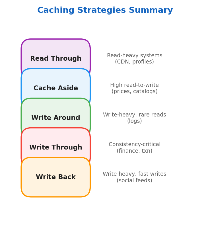
Read Through
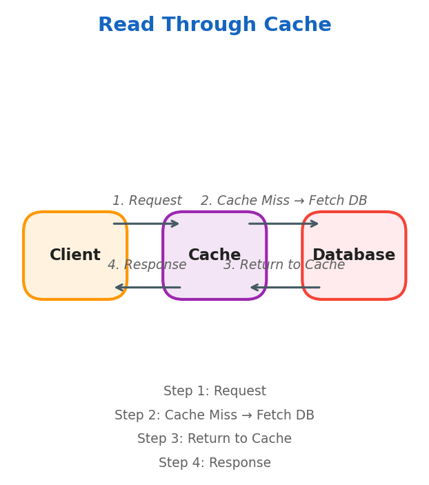
Best for read-heavy systems: CDNs, social media feeds, user profiles.
Cache Aside (Lazy Loading)
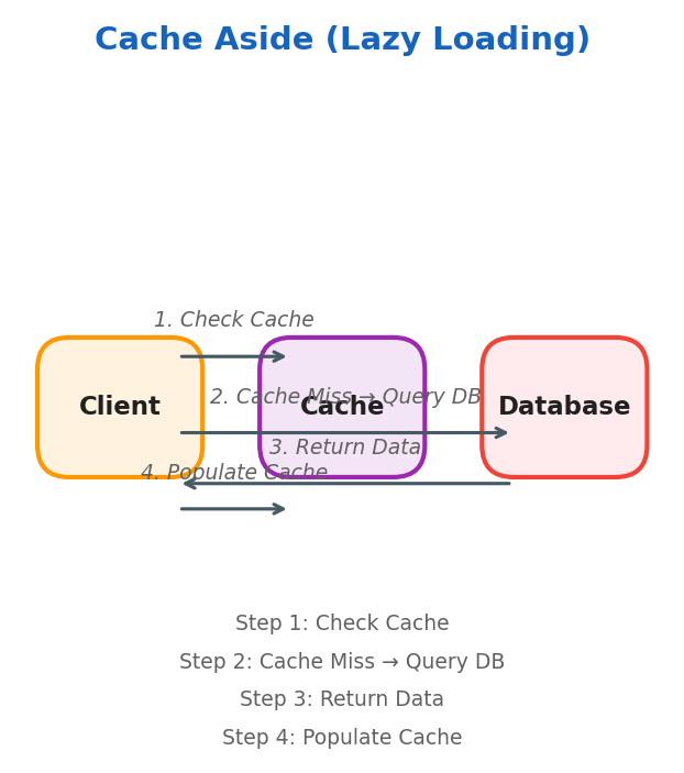
Data is stored in cache only when needed. Best for systems with high read-to-write ratio (prices, descriptions, stock status).
Write Around
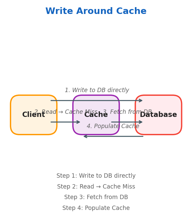
Only frequently accessed data resides in cache. Best for write-heavy systems where data is not immediately read (logging systems).
Write Through
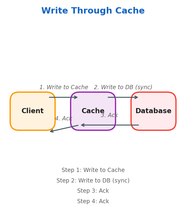
DB and cache are kept in sync. Best for consistency-critical systems, financial applications, online transaction processing.
Write Back
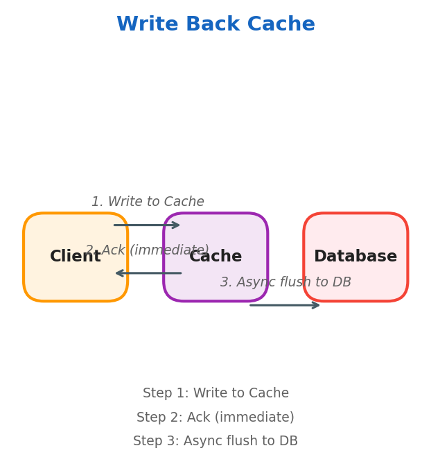
Writes go to cache first, then asynchronously flushed to the database. Ideal for write-heavy scenarios where immediate consistency isn’t critical (logging, social media feeds).
⚠️ Warning: Write-back caching risks data loss if the cache crashes before flushing to the database. Always evaluate your durability requirements before using it.
Strategies Summary
Cache Eviction Policies
Eviction Policies determine which elements are removed when the cache is full.
FIFO (First In, First Out)
Implemented with a queue. The oldest item is evicted first.
LRU (Least Recently Used)
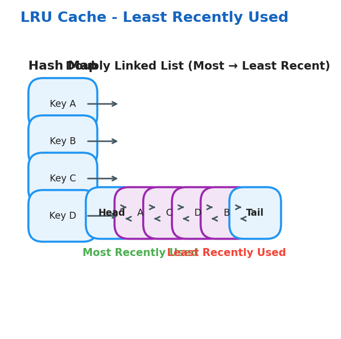
Uses a Hash Map + Doubly Linked List:
- Hash Map: key → pointer to a node in the linked list
- Doubly Linked List: maintains access order (head = most recently accessed)
LFU (Least Frequently Used)
Uses two maps and a frequency tracker:
key_map: key → nodefreq_map: frequency → doubly linked list of nodesmin_freq: integer tracking the minimum frequency
            key_map
    ┌────────────────────┐
    │ A → Node(freq=3)   │
    │ B → Node(freq=1)   │
    │ C → Node(freq=1)   │
    │ D → Node(freq=2)   │
    └─────────┬──────────┘
              │
              ▼
          freq_map
┌─────────────────────────────────┐
│  freq = 1 → [HEAD ⇄ C ⇄ B ⇄ TAIL] │
│              ↑MRU   ↑LRU           │
│  freq = 2 → [HEAD ⇄ D ⇄ TAIL]     │
│  freq = 3 → [HEAD ⇄ A ⇄ TAIL]     │
└─────────────────────────────────┘
  min_freq = 1
Redis Data Structures
Redis is far more than a key-value store:
| Structure | Command | Use case |
|---|---|---|
| String | SET/GET | Simple cache, counters, rate limiting |
| Hash | HSET/HGETALL | User profile, session data |
| List | LPUSH/RPOP | Task queues, activity feeds |
| Sorted Set | ZADD/ZRANGE | Leaderboards, priority queues, time-series |
| HyperLogLog | PFADD/PFCOUNT | Approximate unique visitor counts (±0.81% error) |
| Pub/Sub | PUBLISH/SUBSCRIBE | Real-time notifications, chat |
| Stream | XADD/XREAD | Durable event log, Kafka-lite |
Cache Stampede (Thundering Herd)
When a popular cache key expires simultaneously for many concurrent requests, they all miss and hammer the database at once.
Three mitigations:
- Mutex / single-flight, only one request fetches from DB; others wait for the cached result
- Probabilistic early expiration (PER), slightly before TTL expires, some requests proactively refresh:
import random, math def should_refresh(ttl_remaining, beta=1.0): return -math.log(random.random()) * beta > ttl_remainingbetacontrols refresh aggressiveness (higher beta refreshes earlier/more often; typical values are 0.5–2.0) because-log(random()) * betagrows withbeta, so the expression exceedsttl_remainingmore often. - Background refresh, a background job refreshes cache before TTL expires; serving never misses
💡 Tip: In Go,
singleflight.Groupand in Java, Guava’sLoadingCacheimplement the single-flight pattern out of the box, one request fetches, all others wait for the result.
Cache Invalidation Strategies
💡 Tip: “There are only two hard things in computer science: cache invalidation and naming things.”, Phil Karlton
| Strategy | How it works | When to use |
|---|---|---|
| TTL expiry | Data expires after N seconds | Tolerable staleness, read-heavy |
| Event-driven | Write to DB triggers cache delete/update | Strong consistency requirement |
| Versioned keys | user:123:v4, bump version on write | Immutable deployments, CDN busting |
| Tag-based | Tag cache entries; invalidate by tag | Complex relationships (e.g. all posts by user X) |
Cache Penetration & Bloom Filters
Cache penetration: clients repeatedly query keys that don’t exist in cache or DB (malicious or buggy). Every request falls through to DB.
Mitigation: Bloom Filter, a probabilistic data structure that answers “definitely not in DB” in O(1) with zero false negatives. If the Bloom filter says the key doesn’t exist, skip the DB entirely.
Request key → Bloom Filter check
  ├─ "Definitely not in DB" → return 404 immediately (no DB hit)
  └─ "Maybe in DB" → check cache → check DB
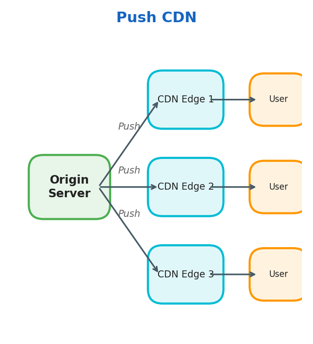
CDN (Content Delivery Network)
CDN Servers are groups of static content cache servers placed close to end users for low latency.
Push CDN
The origin server pushes data to CDN edge nodes proactively.
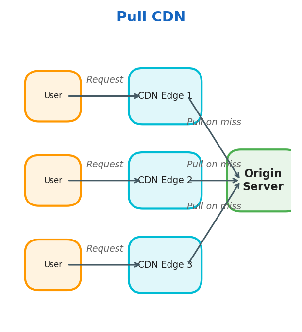
Pull CDN
CDN edge nodes pull data from the origin server on cache miss.
Cache-Control Headers
The origin server instructs CDN and browser caches via Cache-Control:
| Directive | Meaning |
|---|---|
max-age=3600 | Cache for 3600 seconds (client + CDN) |
s-maxage=86400 | CDN caches for 86400s; client uses max-age |
no-cache | Must revalidate with origin before serving |
no-store | Never cache (sensitive data: banking, health) |
stale-while-revalidate=60 | Serve stale while fetching fresh in background |
immutable | Content never changes, skip revalidation entirely (versioned assets: app.v3.js) |
Best practice for static assets: version the filename (main.abc123.js), set Cache-Control: public, max-age=31536000, immutable. Change the filename on every deploy, zero stale content, infinite cache lifetime.
Edge Computing
Modern CDNs run code at the edge, eliminating round-trips to the origin entirely:
- Cloudflare Workers, V8 JavaScript at 300+ edge locations, <1ms cold start
- AWS Lambda@Edge / CloudFront Functions, Node.js or lightweight JS at the CDN layer
- Use cases: A/B testing without origin round-trip, auth token validation, request rewriting, personalised HTML without a server
When NOT to Use a CDN
⚠️ Warning: CDNs hurt more than they help in these cases:
- Highly personalised responses, every user gets unique HTML; CDN hit rate approaches 0%
- Sensitive data, CDN provider can inspect unencrypted content at their edge
- Very high write frequency, data changing faster than TTL means users always get stale content
- Low-latency internal APIs, adding CDN hops increases latency for internal traffic
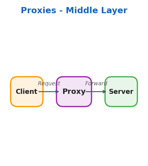
Proxies
Proxies are a middle layer between client and server.
Forward Proxy
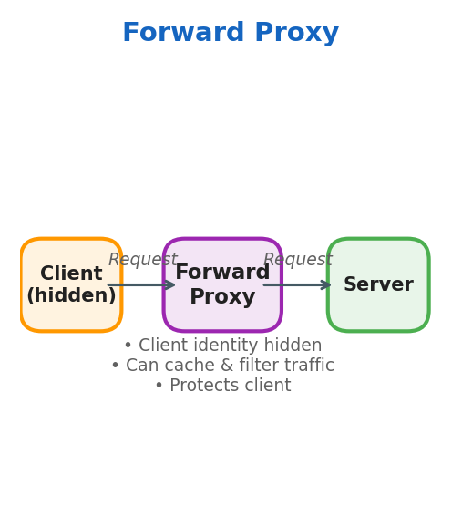
- Client identity is hidden from the server
- Proxy can cache results and filter traffic
- Protects the client
Reverse Proxy
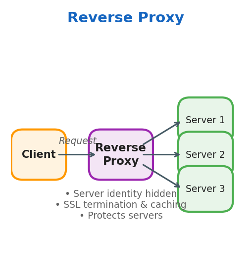
- Server identity is hidden from the client
- Proxy forwards requests to the correct backend server
- Handles SSL termination and caching
- Protects the servers
API Gateway vs Reverse Proxy
These terms are often conflated but have distinct responsibilities:
| Concern | Reverse Proxy | API Gateway |
|---|---|---|
| TLS termination | Yes | Yes |
| Load balancing | Yes | Yes |
| Authentication | No | Yes (JWT, OAuth2, API keys) |
| Rate limiting | Basic | Advanced (per-user, per-plan) |
| Request transformation | No | Yes (header injection, body rewrite) |
| Routing by content | Limited | Yes (route by path, header, body) |
| Analytics / logging | Basic | Detailed per-endpoint |
| Examples | NGINX, HAProxy | Kong, AWS API Gateway, Apigee |
Service Mesh & Sidecar Proxies
At microservice scale, cross-cutting concerns (auth, retries, circuit breaking, tracing) become a tax on every service team. A service mesh moves this logic into a sidecar proxy injected alongside each service container.
┌─────────────────────────────────────────┐
│  Pod A                   Pod B           │
│  ┌──────────┐           ┌──────────┐    │
│  │ Service  │◄─mTLS────►│ Service  │    │
│  └──────────┘           └──────────┘    │
│  ┌──────────┐           ┌──────────┐    │
│  │  Envoy   │           │  Envoy   │    │  ← sidecar proxies
│  │ (sidecar)│           │ (sidecar)│    │
│  └──────────┘           └──────────┘    │
└─────────────────────────────────────────┘
            ▲                   ▲
            └──── Control Plane (Istio / Linkerd) ────┘
What the sidecar handles automatically (zero code changes to the service):
- mTLS between all services (zero-trust networking)
- Distributed tracing (injects trace IDs into every request)
- Circuit breaking and retries with backoff
- Traffic splitting for canary deployments
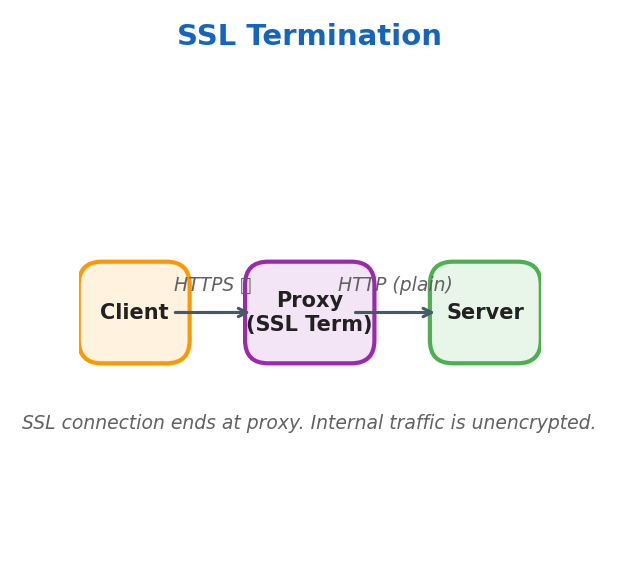
SSL Termination
SSL connection ends at the proxy. Internal traffic from proxy to server uses plain HTTP.
SSL Pass Through
All traffic remains encrypted end-to-end. The proxy forwards encrypted traffic without decrypting.
Load Balancer
A load balancer is a reverse proxy that distributes traffic to backend servers.
Health Checks
A load balancer must know which backends are healthy before routing traffic.
| Type | Mechanism | Pros | Cons |
|---|---|---|---|
| Passive | Detect failures from real request errors (5xx, timeouts) | No extra traffic | Slow to detect, real users see errors first |
| Active | Periodically probe a /health or /ready endpoint | Fast detection | Endpoint must be implemented and meaningful |
Health check config (NGINX example):
upstream backend {
    server app1:8080;
    server app2:8080;
    health_check interval=5s fails=3 passes=2 uri=/health;
}
fails=3, remove backend after 3 consecutive failurespasses=2, re-add backend after 2 consecutive successes (avoids flapping)
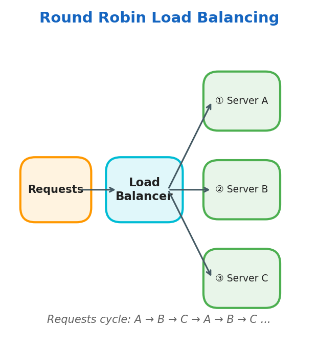
Round Robin
Requests cycle through servers in order: A → B → C → A → B → C…
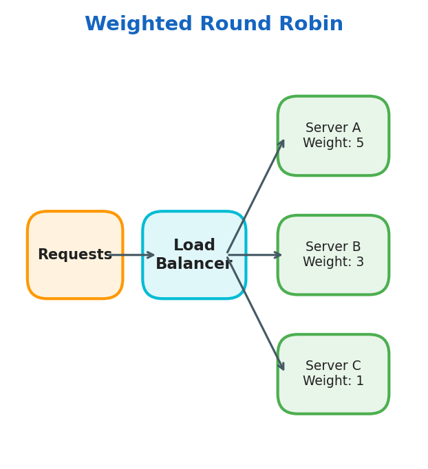
Weighted Round Robin
Same circular pattern, but servers with higher weight receive proportionally more traffic.
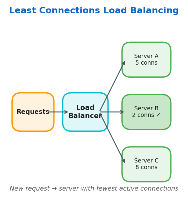
Least Connections
Routes new requests to the server with the fewest active connections.
User Location
Routes based on the user’s geographic location for lowest latency.
Regular Hashing
Same IP always maps to the same server:
$$\text{Dest-Server} = \text{Client-IP} \mod N_{\text{servers}}$$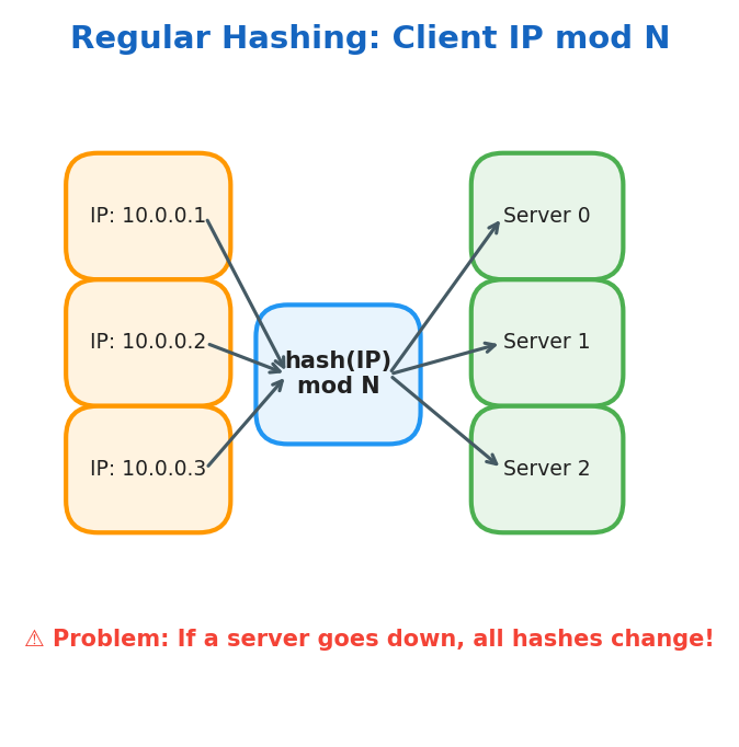
Problem: If a server goes down, all hash mappings need to be recalculated.
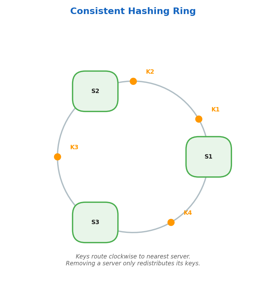
Consistent Hashing
Servers and keys are mapped onto a hash ring. Keys route clockwise to the nearest server. When a server is removed, only its keys are redistributed.
Consistent Hashing Deep Dive
With regular modular hashing, adding or removing a server changes N, so most keys are remapped:
server = hash(key) % N
Consistent hashing places both keys and servers on the same logical ring [0, 2^32). To route a request, hash the key and move clockwise to the next server position on the ring. When a server is added or removed, only nearby key ranges move.
graph TD
    Ring["Hash Ring [0 → 2³²]"]
    Ring --> S1["Server A @ position 10"]
    Ring --> S2["Server B @ position 120"]
    Ring --> S3["Server C @ position 240"]
    S1 --> K1["Key 'user:1' → hash 15\nRoutes to Server A"]
    S2 --> K2["Key 'user:2' → hash 130\nRoutes to Server B"]
    S3 --> K3["Key 'user:3' → hash 250\nRoutes to Server C"]
Virtual nodes (vnodes) map each physical server to multiple ring positions to improve balance. Without vnodes, random placement can make one server own a disproportionately large arc and receive most traffic.
This approach is used in Cassandra, DynamoDB, Amazon load balancing systems, and many Memcached client libraries.
Trade-off: implementation is slightly more complex, but lookup is typically O(log N) with a sorted map or tree structure.
Sticky Sessions
Some stateful applications require that a user’s requests always reach the same server (e.g., servers holding in-memory session state).
Methods:
- Cookie-based: LB injects a
SERVERIDcookie; subsequent requests route to the same server - IP-hash: already covered in the post, but note that it breaks with NAT (many users share one IP)
⚠️ Warning: Sticky sessions undermine the purpose of load balancing, one server can become overloaded if a user’s session is expensive. The better solution is to externalize session state to Redis so any server can handle any request.
Connection Draining
When a backend is being removed (deployment, scale-down), in-flight requests must complete:
- LB marks backend as “draining”, stops sending new connections
- Existing connections are allowed to finish (configurable timeout, e.g. 30s)
- After drain period, backend is removed
Without draining: users experience abrupt mid-request 502 errors on every deployment.
Load Balancer High Availability
The LB itself is a single point of failure. Standard solutions:
- Active-passive: primary LB handles traffic; secondary is on standby. Floating IP (VRRP) moves to secondary on failure. Failover time: 1–5s.
- Active-active: both LBs handle traffic; DNS or anycast routes to either. No failover delay; doubles capacity.
- Cloud-managed LBs (AWS ALB, GCP Cloud Load Balancing): Google/AWS manages HA internally, the LB is not a SPOF from your perspective.
Layer 4 vs Layer 7 Load Balancing
| Type | Level | Speed | Intelligence |
|---|---|---|---|
| Layer 4 | Transport (TCP/UDP) | Faster | Basic routing |
| Layer 7 | Application (HTTP) | Slower | Content-aware routing |
Storage
RDBMS (Relational Databases)
SQL is the language to query relational databases. Data is stored in tables on disk.
B+ Tree Index
Relational databases implement indexing using B+ Trees for O(log n) I/O operations.

Key properties:
- Every node can have m children
- Each node has m-1 values
- Data is stored only on leaf nodes
- Leaf level forms a sorted linked list
- Root/internal nodes are used to efficiently locate data on leaf nodes
| Index Type | Best for | Trade-off |
|---|---|---|
| B+ Tree | Range queries, sorted access | Slower writes |
| Hash Index | Exact-match lookups | No range queries |
| Composite Index | Multi-column WHERE clauses | Column order matters |
| Covering Index | Queries answered entirely from index | More storage |
| Full-Text Index | LIKE / text search | Not for numeric data |
Table Structure
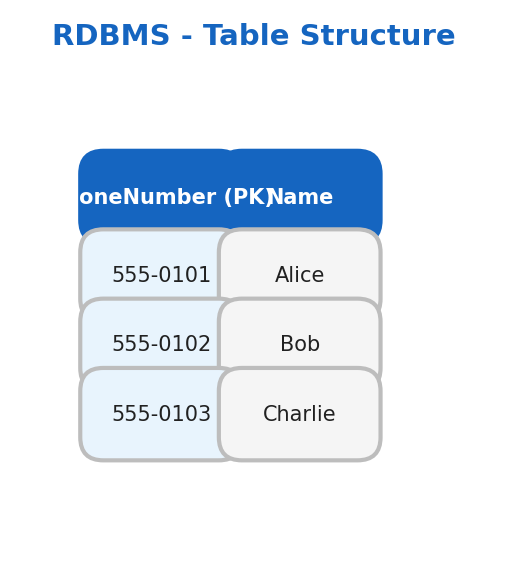
Data Schema defines how data is structured:
CREATE TABLE People (
    PhoneNumber int PRIMARY KEY,
    Name varchar(100)
);
Foreign Keys link two tables together. Joins combine tables based on conditions.
ACID Properties
| Property | Description |
|---|---|
| Atomicity | Transaction is all-or-nothing. If any step fails, the entire transaction rolls back |
| Consistency | Transactions only bring the DB from one consistent state to another |
| Isolation | Concurrent transactions execute as if running in isolation |
| Durability | Once committed, data persists even after system failure (stored on disk) |
Transaction Isolation Levels
ACID’s “Isolation” property has four levels, each a trade-off between correctness and concurrency:
| Level | Dirty Read | Non-Repeatable Read | Phantom Read | Performance |
|---|---|---|---|---|
| Read Uncommitted | Possible | Possible | Possible | Highest |
| Read Committed | Prevented | Possible | Possible | High (Postgres default) |
| Repeatable Read | Prevented | Prevented | Possible | Medium (MySQL InnoDB default) |
| Serializable | Prevented | Prevented | Prevented | Lowest |
⚠️ Warning: Many ORMs (Hibernate, SQLAlchemy) default to Read Committed and do not automatically wrap multi-step operations in a single transaction unless you explicitly define a transaction boundary. Always verify your ORM is actually wrapping writes in a transaction, especially for operations like order creation + inventory decrement.
Definitions:
- Dirty read: reading uncommitted data from another transaction
- Non-repeatable read: re-reading a row mid-transaction returns different values (another TX committed a change)
- Phantom read: re-running a query mid-transaction returns different rows (another TX inserted/deleted)
💡 Tip: Most applications work correctly at Read Committed. Reach for Serializable only when financial or inventory correctness is critical, and test performance carefully, as it can reduce throughput by 10–100×.
MVCC (Multi-Version Concurrency Control)
Modern databases (PostgreSQL, MySQL InnoDB) achieve isolation without blocking reads using MVCC:
- Every row has a
created_atandexpired_attransaction ID - A
SELECTsees a snapshot of all rows that were committed before the transaction started - Writers create a new row version; readers see the old version concurrently
- Result: readers never block writers, writers never block readers
This is why SELECT in Postgres is almost always non-blocking, it reads from a consistent snapshot, not the live data.
sequenceDiagram
    participant T1 as Transaction 1 (reader)
    participant T2 as Transaction 2 (writer)
    participant DB as Database
    T1->DB: BEGIN (snapshot at txn_id=100)
    T2->DB: BEGIN
    T2->DB: UPDATE users SET name='Bob' WHERE id=1
    T2->DB: COMMIT (txn_id=101)
    T1->DB: SELECT name FROM users WHERE id=1
    DB->T1: 'Alice' (sees snapshot at txn_id=100, not 101)
    T1->DB: COMMIT
    Note over T1,DB: T1 read a consistent snapshot, never blocked T2
Write-Ahead Log (WAL)
WAL is the mechanism behind ACID Durability. Before any data page is modified:
- The change is written to an append-only log on disk (the WAL)
- The log entry is
fsync’d, guaranteed to survive a crash - Only then is the in-memory buffer modified and eventually flushed to the data file
On crash recovery: replay the WAL to reconstruct any uncommitted changes. This is also the foundation of replication, replicas stream and replay the WAL from the primary.
📖 Deep Dive: The PostgreSQL WAL documentation explains the full recovery model: https://www.postgresql.org/docs/current/wal-intro.html
LSM-Tree vs B+ Tree
| B+ Tree | LSM-Tree | |
|---|---|---|
| Used by | PostgreSQL, MySQL, SQLite | Cassandra, RocksDB, LevelDB |
| Write path | In-place update (random I/O) | Sequential append to memtable → SSTables |
| Read path | Fast (O(log n) single lookup) | Slower (check multiple SSTables + bloom filters) |
| Write throughput | Moderate | Very high |
| Read throughput | Very high | Good (with bloom filters + caching) |
| Space amplification | Low | Higher (compaction needed) |
| Best for | Mixed read/write, OLTP | Write-heavy, time-series, log storage |
NoSQL
| Type | Description | Examples |
|---|---|---|
| Key-Value | Stores data as key-value pairs | Redis, Memcached, etcd |
| Document | Stores data as JSON documents | MongoDB |
| Wide-Column | Stores data in columns instead of rows | Cassandra, Google Bigtable |
| Graph | Stores data as relationships between objects | Neo4j |
BASE Properties
| Property | Description |
|---|---|
| Basically Available | All users can access the database concurrently |
| Soft State | Data can have multiple intermediate states |
| Eventually Consistent | Consistency is achieved once all replicas are updated |
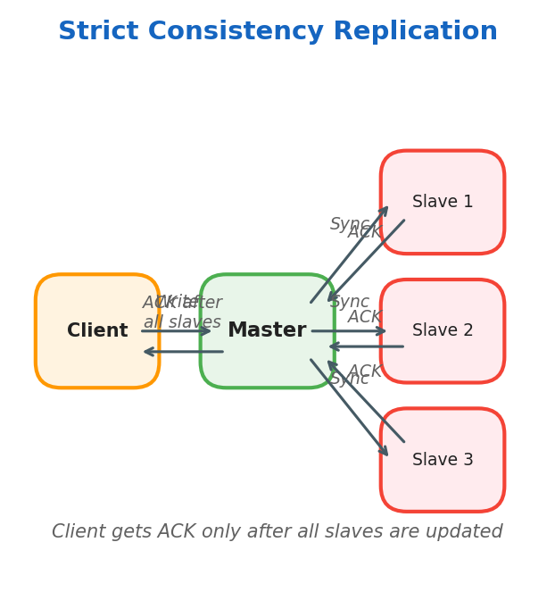
Eventually Consistent vs Strict Consistency
Eventually Consistent: Client writes to the master node and receives ACK immediately. The master node updates slaves asynchronously.
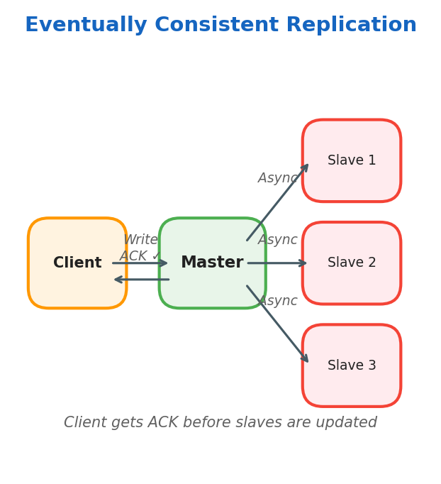
Strictly Consistent: Data is written to the master and immediately copied to all slaves. Client receives ACK only after all slaves confirm.
Replication and Sharding
Synchronous Replication
Master replicates data on slaves at write time. Used when critical consistency is needed.
Asynchronous Replication
Master replicates data on slaves later. Used when consistency can be eventually achieved.
Read Replicas & Replication Lag
Read replicas offload SELECT queries from the primary, but introduce replication lag:
- Synchronous replication: zero lag; every write waits for replica ACK. Adds write latency equal to network RTT to replica.
- Asynchronous replication: near-zero write latency; lag typically <1s on healthy networks but can spike to minutes under high write load.
Application implications:
- After a
POST /orders(write), don’t immediatelyGET /ordersfrom a replica, you may read your own stale write. Use read-your-writes consistency: route reads to the primary for a short post-write window keyed by user/session (size this window from measured replication lag + safety margin), or use a consistency token that forces primary reads until replicas catch up. - Replica lag monitoring: alert if lag exceeds your SLO. Key metric:
seconds_behind_masterin MySQL,pg_stat_replication.write_lagin Postgres.
Master-Master Replication
Multiple masters replicate each other and each replicates its own slaves. Ideal for multi-region setups with one master per region.
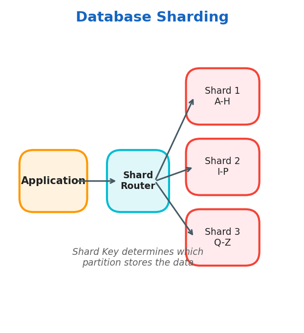
Sharding
Sharding divides data into partitions based on a shard key.
Use cases: massive, high-traffic systems
- Relational databases, sharding is done at the application level
- NoSQL databases, horizontal scaling per shard
| Strategy | How it works | Pros | Cons |
|---|---|---|---|
| Range sharding | Rows with key in [A–M] → Shard 1, [N–Z] → Shard 2 | Simple range queries | Hotspots if data is skewed |
| Hash sharding | shard = hash(key) % N | Uniform distribution | No range queries; resharding is expensive |
| Directory sharding | A lookup table maps keys → shards | Flexible | Lookup table is a SPOF; extra hop |
| Geo sharding | Data partitioned by user geography | Low latency | Cross-region queries are hard |
⚠️ Warning: Avoid sharding until you genuinely need it. It adds enormous operational complexity and makes cross-shard transactions nearly impossible. Try vertical scaling, read replicas, and caching first.
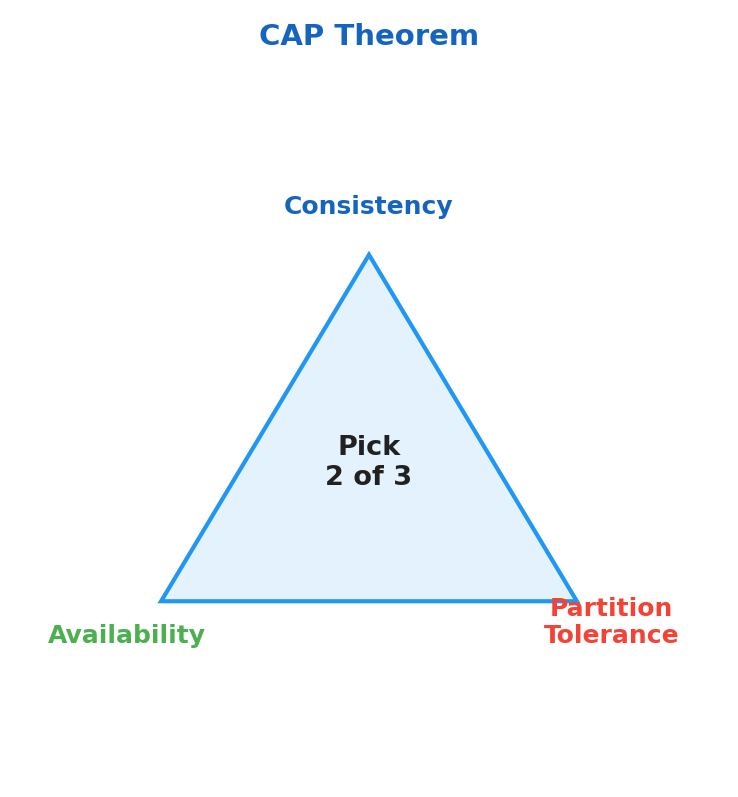
CAP Theorem
In distributed systems, CAP refers to three properties:
- Consistency (C): every read receives the most recent write (or an error), so all nodes present the same logical value.
- Availability (A): every request receives a non-error response, even if that response may not reflect the latest write.
- Partition Tolerance (P): the system continues operating despite network splits where nodes cannot communicate reliably.
graph TD
    CAP{CAP Theorem}
    CAP --> C[Consistency\nAll nodes see same data]
    CAP --> A[Availability\nSystem always responds]
    CAP --> P[Partition Tolerance\nWorks despite network splits]

    C & P --> CP[CP Systems\nZookeeper, HBase,\nPostgreSQL]
    A & P --> AP[AP Systems\nCassandra, CouchDB,\nDynamoDB default]
    C & A --> CA[CA Systems\nOnly possible with\nno partitions]

    style CP fill:#4a90d9,color:#fff
    style AP fill:#e67e22,color:#fff
    style CA fill:#95a5a6,color:#fff
Why can you only guarantee two properties at once? During a network partition, nodes are split into groups that cannot talk to each other. At that moment, you must choose:
- keep serving traffic on both sides (Availability) and risk divergent data (weaken Consistency), or
- reject operations on one side until quorum is restored (Consistency) and sacrifice immediate responses (weaken Availability).
| System | Type | Why |
|---|---|---|
| PostgreSQL / MySQL | CP | Refuses writes during partition to stay consistent |
| Apache Cassandra | AP | Accepts writes during partition, syncs later |
| Apache Zookeeper | CP | Stops accepting writes if quorum is lost |
| CouchDB | AP | Multi-master, eventual consistency |
| HBase | CP | Built on HDFS, prioritizes consistency |
| DynamoDB | AP (tunable) | Adjustable consistency per request |
CAP explains behavior during partitions, but real systems also optimize for normal operation. PACELC extends CAP with latency trade-offs:
if Partition → (Availability vs. Consistency) else (Latency vs. Consistency)
Examples:
- DynamoDB: often described as PA/EL (favoring availability under partition and latency when healthy).
- Spanner: often described as PC/EC (favoring consistency in both partitioned and healthy scenarios).
📖 Deep Dive: Read the original Dynamo paper for a real-world AP system: Amazon Dynamo (2007)
Message Queues & Event Streaming
Asynchronous messaging is a core scaling pattern:
- It decouples producers from consumers.
- It absorbs traffic spikes through buffering.
- It enables fan-out, where one event triggers many downstream services.
| Guarantee | Description | Risk |
|---|---|---|
| At-most-once | Fire and forget | Data loss possible |
| At-least-once | Retry until ACK | Duplicates possible |
| Exactly-once | Idempotent + transactional | Most expensive |
| Feature | Kafka | RabbitMQ | SQS |
|---|---|---|---|
| Model | Log / pull | Queue / push | Queue / pull |
| Ordering | Partition-level | Per-queue | FIFO queue option |
| Retention | Configurable (days/weeks) | Until consumed | Up to 14 days |
| Throughput | Very high | High | High |
| Replay | Yes (seek offset) | No | No |
| Best for | Event streaming, analytics | Task queues, microservices | Serverless, AWS-native |
In Kafka, a consumer group lets multiple consumers share work: each partition is assigned to one consumer in the group, enabling parallel processing without duplicate consumption inside that group.
graph LR
    Producer -->|publish event| Topic[Kafka Topic\norder.placed]
    Topic --> CG1[Consumer Group:\nEmail Service]
    Topic --> CG2[Consumer Group:\nInventory Service]
    Topic --> CG3[Consumer Group:\nAnalytics Service]
    CG1 --> Email[Send confirmation\nemail]
    CG2 --> Inv[Decrease stock\ncount]
    CG3 --> DW[Write to\ndata warehouse]
Observability
Observability tells you not just that a system is failing, but where and why it is failing.
💡 Tip: Instrument your services with OpenTelemetry from day one, it’s vendor-neutral and lets you switch backends (Jaeger, Zipkin, Honeycomb) without changing your code.
The Three Pillars
| Pillar | What it answers | Tool examples |
|---|---|---|
| Logs | What happened? | ELK Stack, Loki, Splunk |
| Metrics | How is the system performing over time? | Prometheus, Datadog, CloudWatch |
| Traces | Where did a request spend its time? | Jaeger, Zipkin, OpenTelemetry |
Golden Signals (Google SRE)
- Latency, time to serve a request (distinguish success vs. error latency)
- Traffic, demand on the system (req/sec)
- Errors, rate of failed requests (4xx/5xx)
- Saturation, how “full” the service is (CPU %, memory %, queue depth)
Prometheus + Grafana Stack
- Prometheus scrapes
/metricsendpoints using a pull model. - Alertmanager fires alerts when thresholds are crossed.
- Grafana visualizes time-series data and dashboards.
from prometheus_client import Counter, start_http_server

REQUEST_COUNT = Counter('http_requests_total', 'Total HTTP requests', ['method', 'endpoint'])

def handle_request(method, endpoint):
    REQUEST_COUNT.labels(method=method, endpoint=endpoint).inc()
    # ... handle request

start_http_server(8000)  # exposes /metrics on port 8000
Further Reading & Resources
📚 Books
- Designing Data-Intensive Applications, Martin Kleppmann, the definitive book on distributed systems
- System Design Interview Vol. 1 & 2, Alex Xu, practical interview preparation
- The Art of Scalability, Abbott & Fisher, organizational and technical scaling
🌐 Free Online Resources
- System Design Primer, 240k+ GitHub stars, comprehensive guide
- ByteByteGo Newsletter, weekly system design deep dives
- Google SRE Book, free, authoritative guide to running production systems
- Martin Fowler, Patterns of Enterprise Architecture, architectural patterns explained
- High Scalability Blog, real-world architecture case studies
📄 Foundational Papers
- Amazon Dynamo (2007), the paper that defined modern AP databases
- Google Bigtable (2006), wide-column store at planetary scale
- Google Spanner (2012), globally distributed CP database
🛠️ Practice
- Excalidraw, whiteboard diagrams for design interviews
- Pramp, free mock system design interviews